Federal R&D Spending on climate change
 Photo by Harrison Moore on Unsplash
Summary
This is a short exploration into the tidy tuesday dataset focused on the Federal R&D budget towards global climate change. The data has been extracted from a TidyTuesday dataset, which in return is moderately cleaned dataset from publicly available data. The analysis will show that NASA’s budget dwarfs the money going into other departments, and that the median spend towards climate change has been increasing since the year 2000.
Useful links:
- Github Repo of Tidy Tuesday explorations
- Tidy tuesday dataset: link
- Data Dictionary link
- Viz posted on Twitter to participate in TidyTuesday.
- Tools used: ESS, Org mode
Download R script : this is the entire script below.
Loading libraries
The easypackages library allows quickly installing and loading multiple packages. Note: Uncomment the appropriate line if this library needs to be installed.
                                        # Loading libraries

                                        # install.packages("easypackages")

library("easypackages")
libraries("tidyverse", "tidyquant", "DataExplorer")
All packages loaded successfully
Reading in the data
Since this is a small dataset, the data can be read in directly from Github into memory.
                                        # Reading in data directly from github

climate_spend_raw  <- readr::read_csv("https://raw.githubusercontent.com/rfordatascience/tidytuesday/master/data/2019/2019-02-12/climate_spending.csv", col_types = "cin")
Exploring the data
We have 6 departments, and the remaining departments are lumped together as ‘All Other’.
The data is available for the years 2000 to 2017.
The above can be found using the unique function.
climate_spend_raw$department %>% unique()
climate_spend_raw$year %>% unique()
[1] "NASA"            "NSF"             "Commerce (NOAA)" "Energy"
[5] "Agriculture"     "Interior"        "All Other"

 [1] 2000 2001 2002 2003 2004 2005 2006 2007 2008 2009 2010 2011 2012 2013 2014
[16] 2015 2016 2017
Some Notes on the data:
- We have the following columns:
- name of the department. (chr)
- year (int)
- spending (double)
- The data is relatively clean. However some manipulation is required to summarise the department wise spending.
An overview of missing data can be easily scrutinised using the plot_intro command, and actual numbers can be extracted using introduce. These functions are from the DataExplorer package.
##plot_str(climate_spend_raw, type = 'r')

plot_intro(climate_spend_raw)
##introduce(climate_spend_raw)
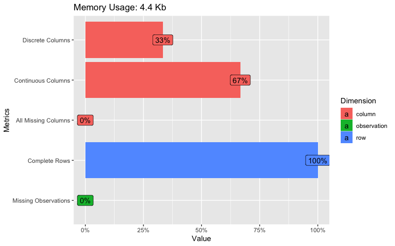
There are no missing values or NA’s.
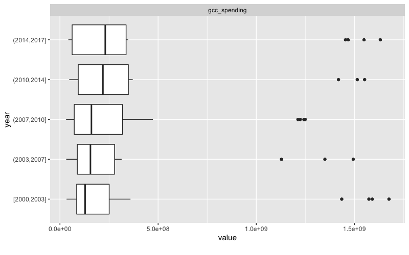
For a quick look at the outliers, we can use a boxplot, using DataExplorer’s functions.
variance_climate_spend <- plot_boxplot(climate_spend_raw, by = "year")
Data Conditioning
Note: this initial conditioning need not have involved the date manipulation, as the year extracted from a date object is still a double.
climate_spend_conditioned <- climate_spend_raw %>%
  mutate(year_dt = str_glue("{year}-01-01")) %>%
  mutate(year_dt = as.Date(year_dt)) %>%
  mutate(test_median = median(gcc_spending)) %>%
  mutate(gcc_spending_txt = scales::dollar(gcc_spending,
                                           scale = 1e-09,
                                           suffix = "B"
                                           )
         )
Applying some summary statistics to calculate the total spend per department, per year.
                                        # Total spend per department per year

climate_spend_dept_y <- climate_spend_conditioned %>%
  group_by(department, year_dt = year(year_dt)) %>%
  summarise(
    tot_spend_dept_y = sum(gcc_spending)) %>%
  mutate(tot_spend_dept_y_txt = tot_spend_dept_y %>%
           scales::dollar(scale = 1e-09,
                          suffix = "B")
         ) %>%
  ungroup()
Lets see how much money has been budgeted in each department towards R&D in climate change from 2000 to 2017.
climate_spend_conditioned %>%
  select(-c(gcc_spending_txt, year_dt)) %>%
  group_by(department) %>%
  summarise(total_spend_y = sum(gcc_spending)) %>%
  arrange(desc(total_spend_y)) %>%
  mutate(total_spend_y = total_spend_y %>% scales::dollar(scale = 1e-09,
                                                        suffix = "B",
                                                        prefix = "$")
       )
| Department | Total Spend from 2000-2017 |
|---|---|
| NASA | $25.77B |
| Commerce (NOAA) | $5.28B |
| NSF | $5.26B |
| Energy | $3.32B |
| Agriculture | $1.63B |
| All Other | $1.54B |
| Interior | $0.86B |
It is clear from here that the outlier department is NASA. Further exploration would be needed to understand the function of each department and the justification of this expenditure and the skew. For example, one might think the Interior department would not be able to produce R&D superior to NASA/NSF.
Function to plot a facet grid of the department spending
By using a function to complete the plot, the plot can be easily repeated for any range of years. It can also work for a single year.
The function below takes the following arguments:
- The range of the years we want to look into , example 2005-2010
- The number of columns in the facet wrap plot.
- The caption that consititues the observation from the plots and anything else.
The title of the plot includes the year range that is input above.
climate_spend_plt_fn <- function(
data,
y_range_low = 2000,
y_range_hi = 2010,
ncol = 3,
caption = ""
)
{
plot_title <- str_glue("Federal R&D budget towards Climate Change: {y_range_low}-{y_range_hi}")
data %>%
filter(year_dt >= y_range_low & year_dt <= y_range_hi) %>%
ggplot(aes(y = tot_spend_dept_y_txt, x = department, fill = department ))+
geom_col() +
facet_wrap(~ year_dt,
ncol = 3,
scales = "free_y"
) +
#scale_y_continuous(breaks = scales::pretty_breaks(10)) +
theme_tq() +
scale_fill_tq(theme = "dark") +
theme(
axis.text.x = element_text(angle = 45,
hjust = 1.2),
legend.position = "none",
plot.background=element_rect(fill="#f7f7f7"),
) +
labs(
title = plot_title,
x = "Department",
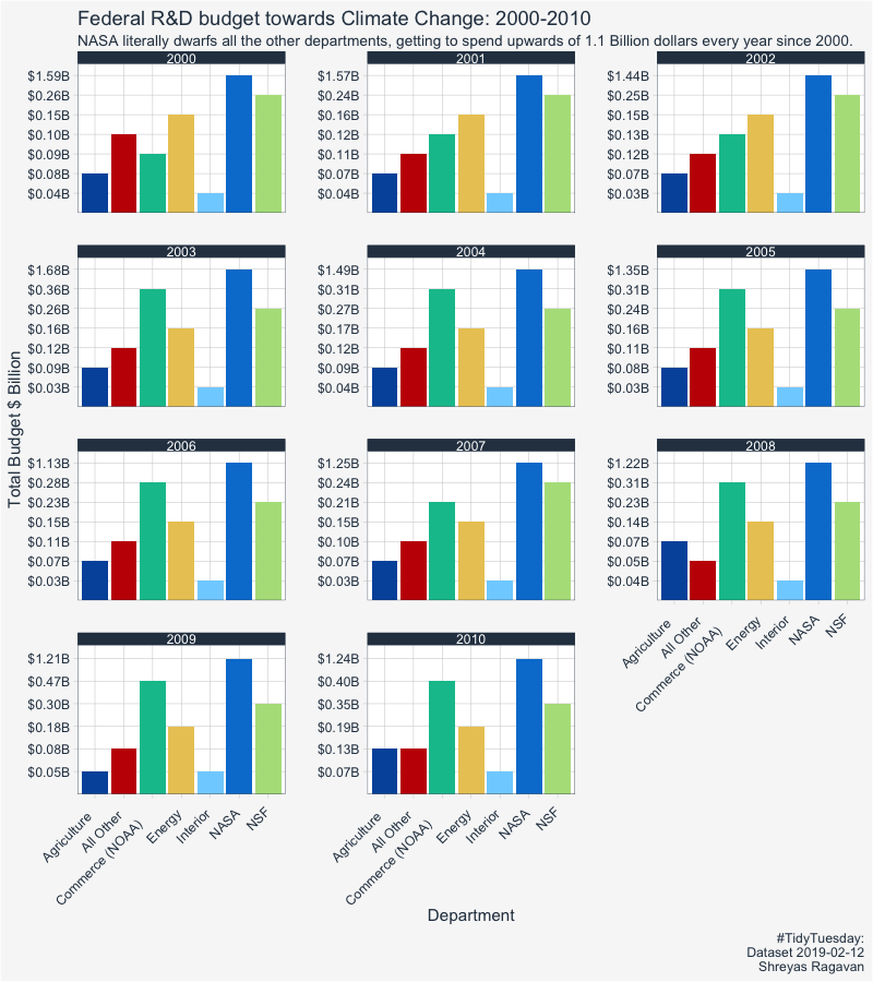
y = "Total Budget $ Billion",
subtitle = "NASA literally dwarfs all the other departments, getting to spend upwards of 1.1 Billion dollars every year since 2000.",
caption = caption
)
}
Visualizing department-wise spending over the years
Calling the function and passing in the entire date (year) range of 2000-2010. Note that for a single year, have both the arguments y_range_low and y_range_high equal to the same year.
climate_spend_plt_fn(climate_spend_dept_y,
                     y_range_low = 2000,
                     y_range_hi = 2010,
                     caption = "#TidyTuesday:\nDataset 2019-02-12\nShreyas Ragavan"
                       )
climate_spend_plt_fn(climate_spend_dept_y,
                     y_range_low = 2011,
                     y_range_hi = 2017,
                     caption = "#TidyTuesday:\nDataset 2019-02-12\nShreyas Ragavan"
                       )

Some Concluding statements
NASA has the highest R&D budget allocation towards climate change, and one that is significantly higher than all the other departments put together. The median spending on R&D towards climate change has been increasing over the years, which is a good sign considering the importance of the problem. Some further explorations could be along the lines of the percentage change in spending per department every year, and the proportion of each department in terms of percentage for each year.